bernstein-von mises theorem & power posteriors

Hey all! Hope you are doing well. In this post, I aim to cover some results regarding Bayesian inference in model misspecification settings and then actually test them with a short simulation. Let us establish some preliminaries: consider any parameter estimation procedure (e.g. MoM, MLE, MAP) which posits \(X_1, \dots, X_n \overset{\text{i.i.d}}{\sim} f(x \mid \theta)\) whereas in truth \(X_1, \dots, X_n \overset{\text{i.i.d}}{\sim} g\) for some unknown \(g\).

Recall that MLEs \(\hat{\theta}\) have a well-studied asymptotic distribution in this situation, the sandwich variance¹. Written for the univariate case, this can be given by²:

\[\sqrt{n}[\hat{\theta} - \theta^*] \overset{d}{\to} \mathcal{N}(0, \frac{\mathbb{E}_g[(\frac{\partial}{\partial \theta} \log f(X \mid \theta^*))^2]}{\mathbb{E}_g[\frac{\partial^2}{\partial \theta^2} \log f(X \mid \theta^*)]^2}) \quad \theta^* = \underset{\theta}{\mathrm{argmin}} \ \text{KL}(g(x) \mid\mid f(x \mid \theta))\]

as per this short derivation. For notation purposes, let us define this sandwich variance as \(V_{\text{sand}}\). But what about for bayesian inference? As per standard bayesian inference, suppose we assume \(\theta\) is modeled by random variable \(\Theta\) which follows some specified prior. The Bernstein-von Mises theorem tells us that in cases of correct model misspecification, informally for large \(n\), we can write \(\Theta \mid \textbf{X} \overset{\mathrm{approx}}{\sim} \mathcal{N}(\hat{\theta}, \frac{1}{nI(\hat{\theta})})\) where \(I(\theta)\) is the Fisher Information. In cases of model misspecification, Bernwise-von Mises theorem provides an adjustment of the kind we would expect:

\begin{equation} \sqrt{n}[\Theta - \theta^* \mid \mathbf{X}] \overset{d}{\to} \mathcal{N}(0, V_{\text{sand}}) \label{bvm-misspecified} \end{equation}

Nice! We have some understanding of how our posteriors will look in the case of model misspecification, albeit only asymptotically. But what if we could control the rate at which our (misspecified) posterior adjusts to new data? In other words, what if we could make the convergence of \(\Theta \mid \mathbf{X}\) to \eqref{bvm-misspecified} slower.

power posteriors

This is where power posteriors, a rather new method, come into play. For a power posterior \(\Theta \mid \mathbf{X}\) where $\Theta$ is distributed according to prior \(f_{\Theta}(\theta)\), the posterior PDF is given by:

\[f_{\Theta \mid \mathbf{X}}(\theta \mid \mathbf{X}) = \frac{f_{\mathbf{X} \mid \Theta}(\mathbf{X} \mid \theta)^{\gamma} f_{\Theta}(\theta)}{f(X)} = \frac{f_{\Theta}(\theta) \prod_{i = 1}^n f(x_i \mid \theta)^{\gamma}}{\int_{\Theta} f_{\mathbf{X} \mid \Theta}(\mathbf{X} \mid \theta')^{\gamma} f_{\Theta}(\theta') d\theta' } , \quad \quad \gamma \in [0, 1]\]

The intuitive idea is to decrease the weightage of the likelihood terms by raising them to some power \(\gamma \leq 1\) (note for \(\gamma = 1\) this is just our normal posterior).

Note that there have been three discussed interpretations of the power posterior. While we won’t derive them from theory, one that I like and makes intuitive sense is that the power posterior reduces the sample size from \(n\) to \(n\gamma\) (essentially we will need more samples to get the same concentrated (power) posterior³.)

Finally, it has been found that power posteriors do have nice asymptotics. In this paper, they were able to find that power posteriors do converge to the limiting distributions of Bernstein-von Mises Theorem.

worked model misspecification example

We conclude this blog post with some visualizations of these concepts in action, starting with Bernstein-von Mises Theorem. Let us assume we have samples \(X_1, \dots, X_n\) which are truly distributed by $\text{Gamma}(3, 2)$. Note that we are using the shape-rate parametrization of the Gamma distribution for this blog post. Now for the model misspecification: we assume our data is distributed by \(\text{Expo}(\lambda)\) and set a prior $\lambda \sim \text{Gamma}(1, 1)$. Through standard Bayesian Inference, we arrive at the following clean posterior:

\[\lambda \mid \mathbf{X} \sim \text{Gamma}(1 + n, 1 + \sum_{i = 1}^n X_i)\]

We aim to show that this posterior follows our established result \eqref{bvm-misspecified}. To do so, we must compute the pseudo-true value \(\lambda^*\). We provide a quick derivation below, where $g(x)$ gives the true PDF for $\text{Gamma}(3, 2)$:

\[\text{KL}(g(x) \mid\mid f(x \mid \lambda)) = \mathbb{E}_g[\log \frac{g(x)}{f(x \mid \lambda)}] = \mathbb{E}_g[\log g(x)] - \mathbb{E}_g[\log f(x \mid \lambda)]\] \[\implies \lambda^* = \underset{\lambda}{\mathrm{argmin}} \ \ \mathbb{E}_g[\log f(x \mid \lambda)] = \underset{\lambda}{\mathrm{argmax}} \ \ \mathbb{E}_g[\log (\lambda) - \lambda x] = \underset{\lambda}{\mathrm{argmax}} \ \ \log(\lambda) - \lambda\mathbb{E}_g[x]\] \[\implies \lambda^{*} = \frac{1}{\mathbb{E}_{g}[x]} = \frac{1}{\frac{3}{2}} = \frac{2}{3}\]

We can now show the below visualization demonstrating Bernstein-von Mises Theorem as we increase \(n\):

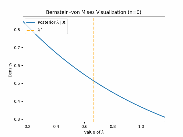
Thus, we can see that our posterior \(\lambda \mid \mathbf{X}\) does indeed converge in distribution to a normal around \(\lambda^*\).

We move onto trying to visualize power posteriors, specifically the effect of \(\gamma\). To do so, we’ll need to derive the derivation of our posterior, for any value of \(\gamma\). We start with our posterior distribution PDF:

\[f_{\mathbf{\lambda} \mid \mathbf{X}}(\lambda \mid \mathbf{X}) \propto f_{\mathbf{\lambda}}(\lambda) \prod_{i = 1}^n f(x_i \mid \lambda)^{\gamma} \implies f_{\mathbf{\lambda} \mid \mathbf{X}}(\lambda \mid \mathbf{X}) \propto e^{-\lambda} \prod_{i = 1}^n \lambda^{\gamma} e^{-\lambda \gamma x_i}\] \[\implies f_{\mathbf{\lambda} \mid \mathbf{X}}(\lambda \mid \mathbf{X}) \propto \lambda^{n\gamma} \text{exp}(-\lambda(1 + \gamma \sum_{i = 1}^n x_i))\]

and so we can conclude $\lambda \mid \mathbf{X} \sim \text{Gamma}(n\gamma + 1, 1 + \gamma \sum_{i = 1}^n x_i)$. Thus for any specified value of \(0\leq \alpha \leq 1\), we have a neat form of the power posterior distribution. Note that if you compare this to the form of our previously derived posterior, the “reducing the sample size” interpretation of power posteriors becomes blatantly clear. We now provide a similar animation as before to show how quickly the (power) posterior(s) converge normally around \(\lambda^*\) as \(n\) increases.

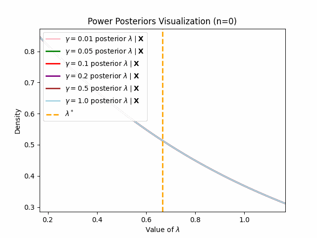
This behavior matches what we should expect (as per the preivously discussed asymptotic result of power posteriors): lower values of \(\gamma\) will engender posteriors which adapt to new observations slower.

code

The code for generating the first visualization showing Bernstein-von Mises Theorem can be found here. Code for visualization of power posteriors can be found here.

sources

Power posteriors are not a frequently discussed topic, so I am super grateful to the below resources:

1. This talk from Jeff Miller on understanding the power posterior
2. This paper whch gives the two really nice results on power posterior asymptotics
3. This blog article on power posteriors which also provided some nice visualizations

Thank you for reading this blog post. If you have any questions or noticed any errata, please email me.