what if we didn't approximate posteriors?

TLDR: Comparing predictive distributions from posteriors estimated by coordinate-ascent variational inference (CAVI) versus exact derivation in a univariate bayesian linear regression setting.

Hey all! Just finished my freshman year of college and thought it would be fun to explore one of the things we learned in my statistical inference class in more depth. Specifically, I am interested in exploring bayesian inference by exploring predictive distributions.

bayesian neural networks: why, what, how

At a high level, bayesian neural networks help us understand the distribution of parameters our model could have taken, conditional on some observed data. This contrasts with standard neural networks, which only focus on learning the optimal parameters (at the risk of overfitting). In other words, given some data $D$ and a model with parameter weights $\theta$, BNNs aim to compute the posterior:

for some chosen prior distribution $p(\theta)$. Setting aside how BNNs actually find this posterior (the subject of this blog post), this posterior then lets us compute predictive distributions for new inputs. For a test point $x$, we have:

We now get into the computability issue for the posterior. As is likely no surprise, the evidence term $p(D)$ in the denominator is usually intractable once $\theta$ is high-dimensional. Two classes of methods are typically used to approximate the posterior: (1) Markov Chain Monte Carlo (MCMC) algorithms like Metropolis Hastings (which exploits the fact that $p(\theta \mid D) \propto p(D \mid \theta)\,p(\theta)$ from Bayes’ Rule) and (2) variational inference which approximates $p(\theta \mid D)$ by learning a surrogate function $q_{\phi}(\theta)$ parametrized by weights $\phi$. For our purposes, we focus on (2) in this article as (1) is often computationally expensive when $\theta$ is high dimensional. While an entire paper can be written on variational inference, we give a brief explanation here.

For our purposes let us assume each weight in $\theta$ is independent from each other and has zero covariance. Variational Inference works by learning weights $\phi$ to minimize the KL divergence between distribution $q_{\phi}(\theta)$ and our posterior $p(\theta \mid D)$. Note however that we cannot directly minimize this KL divergence due to its intractable $p(D)$ term, as shown below¹:

Because $\log p(D)$ is just a constant, it is sufficient to minimize this KL by maximizing the evidence lower bound (ELBO):

While plenty of methods exist for doing this, we can focus on one by making the strong assumption that each parameter in $\theta$ has its own independent distribution. Such a assumption brings us to the land of mean-field variational inference, where we factorize our approximate posterior $q_{\phi}(\theta)$ into:

where each $q_{\phi_i}$ is our estimated PDF of parameter $\theta_i$ parametrized by weights $\phi_i$. Using this form lends itself nicely to Coordinate Ascent Variational Inference (CAVI), where we iteratively maximize the ELBO with respect to one factor ($\phi_i$) while holding the others fixed. CAVI is quite a non-trivial algorithm, and we’ll explore it more when we use it later².

Now, given this fully‐trained approximate stand‐in distribution $q_{\phi}(\theta)$ for the true posterior $p(\theta \mid D)$, we can compute predictive distributions as defined before. Instead of tackling that integral directly, we typically use Monte Carlo integration: sampling i.i.d. parameters $q_{\phi}(\theta)$ and averaging their predictions.

what we’re curious about

Regardless of the choice of MCMC or variational inference, the bottom line is that the posterior distribution is always approximated. But what if we could exactly pinpoint the true posterior? I am interested in comparing predictive distributions from an approximate CAVI-trained posterior versus an exactly computed posterior. Specifically, we will inspect this in the case of univariate (bayesian) linear regression.

step one: defining the problem statement

Let us first define our data $D$ in matrix form as:

where $\epsilon \sim \mathcal{N}(0, \sigma^2) $ for some known $\sigma^2$. Note that we are treating observations $x_1, \dots, x_n$ as fixed. We place the following multivariate normal prior on $\beta$:

for some chosen $\tau_0, \tau_1$. For convenience, we’ll choose $\tau_0 = \tau_1 = 1$ and so we’ll model $\beta$ with the multivariate standard normal distribution $\mathcal{N}(\mathbf{0}, \mathbf{I})$. Furthermore, we’ll set the true residual variance $\sigma^2$ to one and assume it is known. We are now ready to start coding! Let us define this function to generate $D$ from:

import numpy as np
from scipy import stats

SIGMA_SQUARED = 1

# generate D
def generate_data(n=100):
    beta_0_true = np.random.random() * 3
    beta_1_true = np.random.random() * 3
    X = np.random.normal(0, 1, n)
    eps = np.random.normal(0, SIGMA_SQUARED, n)
    y = beta_0_true + beta_1_true * X + eps
    return X, y

Note that this generation process does generate a linear relationship with a (likely) non-trivial difference from its prior.

We now cover the two ways to obtain our posterior $p(\beta \mid D)$: deriving the exact posterior or approximating it with variational inference. We start with the former.

step two: deriving the exact posterior

I cheated a little bit. Our current univariate linear regression problem is a well-studied problem of bayesian linear regression (BLR) where the exact posterior of parameters $\beta$ is well-known. Deriving this exact posterior does require some matrix algebra, but just for completeness we provide a quick derivation (following these class slides). For a more thorough derivation that goes through the complete-the-square trick below, see this excellent Medium article.

where we define $\mu = \tfrac{1}{\sigma^2} \Sigma(X^Ty)$ and $\Sigma^{-1} = \tfrac{1}{\sigma^2} X^TX + S^{-1}$. Note that our last line shows that $p(\beta \mid D)$ takes the form of a multivariate normal distribution, namely we can express:

This concludes the derivation for the exact posterior distribution. It’ll be helpful to implement a function to sample from this posterior (we’ll see why in step three):

S = np.array([[1, 0], [0, 1]])
def sample_from_blr_posterior(X, y, num_samples=1000):
    X_expanded = np.ones((X.shape[0], 2))
    X_expanded[:, 1] = X

    Sigma = np.linalg.inv((1 / SIGMA_SQUARED) * np.matmul(X_expanded.T, X_expanded) + np.linalg.inv(S))
    mu = (1 / SIGMA_SQUARED) * np.matmul(Sigma, np.matmul(X_expanded.T, y))

    return np.random.multivariate_normal(mean=mu, cov=Sigma, size=num_samples)

Note that we are assuming knowledge of $\sigma^2$, the residual variance (as opposed to estimating it.) We are ready to try the second method to obtain our posterior!

step two (and a half): approximating the posterior with variational inference

Let us first establish the form of our stand-in distribution $q_{\phi}(\theta)$ with the (correct) assumption that $\beta_0$ and $\beta_1$ are independent $\implies$ we can use mean-field variational inference and thus represent $q_{\phi}(\beta) = q_{\phi_0}(\beta_0) \times q_{\phi_1}(\beta_1)$. We choose to define $q_{\phi_0}(\beta_0)$ and $q_{\phi_1}(\beta_1)$ by:

where $m_j, s_j^2$ are our learnable parameters. Expressed differently, this form of the approximated posterior posits each $\beta_j$ has its independent normal distribution or that each $\beta_j \sim \mathcal{N}(m_j, s_j^2)$. As previously mentioned, the procedure to now optimize $q_{\phi}(\theta)$ is Coordinate-Ascent Variational Inference (CAVI). While deriving CAVI is above my paygrade, at a high level CAVI aims to iteratively optimize the ELBO w.r.t to one mean-field posterior $q_{\phi_j}(\beta_j)$ while keeping all other posteriors $q_{\phi_{-j}}(\beta_{-j})$ fixed. Specifically, in a given CAVI iteration, we iterate through all parameters and update the $j$th parameter set $\phi_j$ s.t. the following condition is met:

where \(\mathbb{E}_{-j}\) means that we assume \(\forall i \neq j, \beta_i \sim q_{\phi_i}(\beta_i)\). Comparing this condition and our previous ELBO derivation, we can see that it does sort of set $q_{\phi_j}(\beta_j)$ in a way that optimizes an ELBO adjusted for single coordinate optimization. For a formal treatment of how this maximizes the ELBO, see these lecture notes. We now apply this CAVI algorithm to our defined problem by finding how we should update our parameter sets $\phi_0 = (m_0, s_0^2)$ and $\phi_1 = (m_1, s_1^2)$ at each iteration to satisfy our aforementioned condition. Before doing so, it will be helpful to compute \(\log p(\beta, y)\), or equivalently \(\log p(\beta, y \mid x)\) as we are treating \(\mathbf{x}\) as fixed:

Because $S^{-1} = \text{diag}(\tau_0^{-2}, \tau_1^{-2})$, we can compactly represent this as:

For short hand, we refer to the above expression as \(\log p(\beta, y)\). We are now ready to derive the update rule for $\phi_0$. For $\phi_0$, we must satisfy the following condition with our new approximated posterior \(q_{\phi_0}^*(\beta_0)\):

We express a meaningful additive proportionality relationship of \(\mathbb{E}_{q_1} [\log p(\beta, y)]\) below, disregarding constants w.r.t to \(\beta_0\). For our purposes, let \(\propto'\) define additive proportionality (i.e. $x \propto’ y \implies x = y + \text{const}$):

Note that by our update condition, we must have \(\log[q_{\phi_0}^*(\beta_0)]\) additively proportional to our above derived expression. Our above expression matches the log-density form of \(\mathcal{N}(m_{0, *}, s_{0, *}^{2})\) where we define:

and so this serves as our update rule for $q_{\phi_0}(\beta_0)$. We now derive the update rule for \(q_{\phi_1}(\beta_1)\), albeit slightly more tersely this time:

This matches the log density of $\mathcal{N}(m_{1, *}, s_{1, *}^2)$ where we define:

So we have derived the update rules to perform CAVI. All that is left is to actually code these updates, which shouldn’t be too bad:

TAU_0_SQUARED = TAU_1_SQUARED = 1
def beta_0_update(X, y, phi_1):
    m_1 = phi_1[0] # treat as fixed
    n = X.shape[0]
    s_0_new = 1 / ((1 / TAU_0_SQUARED) + (n / SIGMA_SQUARED)) # s_{0, *}^2
    m_0_new = (s_0_new / SIGMA_SQUARED) * np.sum(y - X * m_1)
    return (m_0_new, s_0_new)


def beta_1_update(X, y, phi_0):
    m_0 = phi_0[0]
    s_1_new = 1 / ((1 / TAU_1_SQUARED) + (np.sum(np.pow(X, 2)) / SIGMA_SQUARED)) # s_{1, *}^2
    m_1_new = (s_1_new / SIGMA_SQUARED) * np.sum(X * (y - m_0))
    return (m_1_new, s_1_new)

From here writing the CAVI algorithm to learn $\phi$ is a piece of cake:

def run_cavi(X, y):
    phi_0, phi_1 = [0, 1], [0, 1]
    phi_0, phi_1 = np.array(phi_0), np.array(phi_1)
    while (True):
        phi_0_new = beta_0_update(X, y, phi_1)
        phi_1_new = beta_1_update(X, y, phi_0_new)
        if (np.sum(np.abs(phi_0_new - phi_0)) < 1e-12):
            break
        phi_0 = phi_0_new
        phi_1 = phi_1_new
    return phi_0, phi_1

Similar to how we wrote sample_from_blr_posterior(beta, X, y) function to sample from our exact posterior, we’ll do the same to sample \(\beta\) from our CAVI posterior:

# evaluate q_{phi}(beta) by first learning phi
def sample_from_cavi_posterior(X, y, num_samples=1000):
  phi_0, phi_1 = run_cavi(X, y)
  beta_0_samples = np.random.normal(loc=phi_0[0], scale=np.sqrt(phi_0[1]), size=num_samples)
  beta_1_samples = np.random.normal(loc=phi_1[0], scale=np.sqrt(phi_1[1]), size=num_samples)
  return np.column_stack((beta_0_samples, beta_1_samples))

step three: comparing predictive distributions

The hard part is behind us: we have now been able to learn the posterior \(\beta \mid D\) through two ways: (1) exact posterior derivation and (2) CAVI. Our goal now is to compare how (1) vs. (2) stack up in terms of forming predictive distributions. Recall that our predictive distribution for some fixed test point \(x\) can be given as

and is typically approximated via Monte Carlo integration³. As we’ll see, we use empirical confidence intervals instead to estimate the predictive distribution.

We first generate $n = 1000$ data points using our generate_data function. We plot the data below along with its line of best fit (orange):

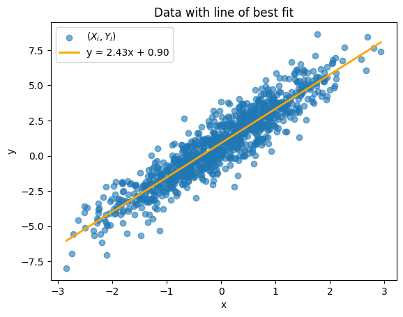
We now present our concrete procedure to compare predictive distributions: for any fixed point \(x\) we sample \(K = 1000\) potential \(\beta\)s from our choice of posterior. Then⁴, for each \(\beta_i\) we sample $\hat{y}$ using its conditional distribution \(\hat{y} \mid x, \beta_i \sim \mathcal{N}(x\beta_i, \sigma^2)\) where \(\sigma^2 = 1\). From these set of \(K\) sampled predictions, we can compute the predicted mean and form an empirical 95% confidence interval for the true \(\hat{y}\). This gives us the predictive distribution confidence interval.

We visually show this procedure below for at \(x = 0\) by plotting the 95% predictive distribution confidence intervals computed from the exact BLR posterior (blue) and the CAVI-learned posterior (green).

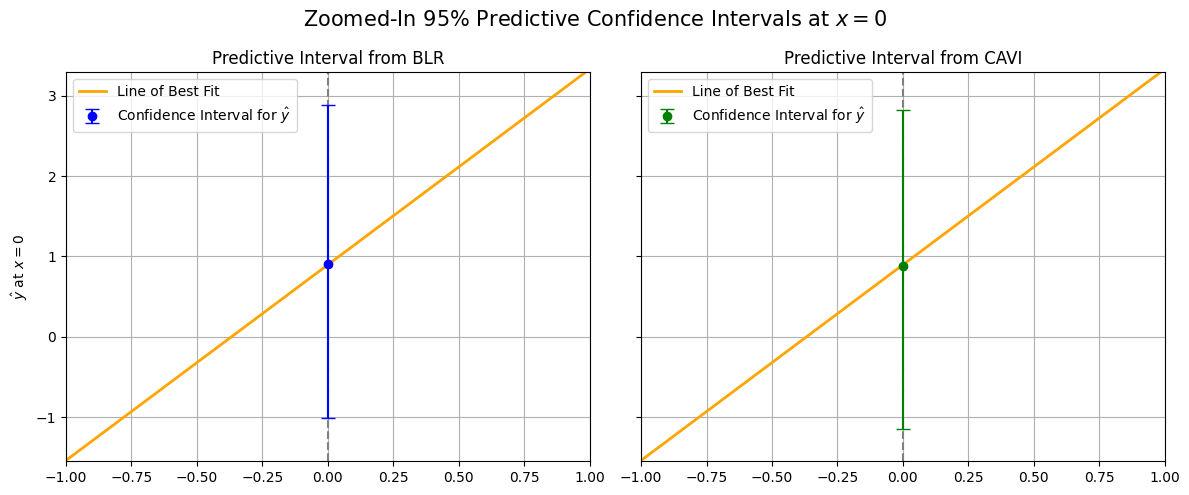
We can see that the widths and placements of the predictive confidence intervals themselves are nearly identical, and both predicted means (the dots) are pretty close to the line of best fit. We now repeat this exact same procedure to compare predictive distribution confidence intervals across 1000 different choices of \(x\) from \([-3, 3]\), all in the same plot:

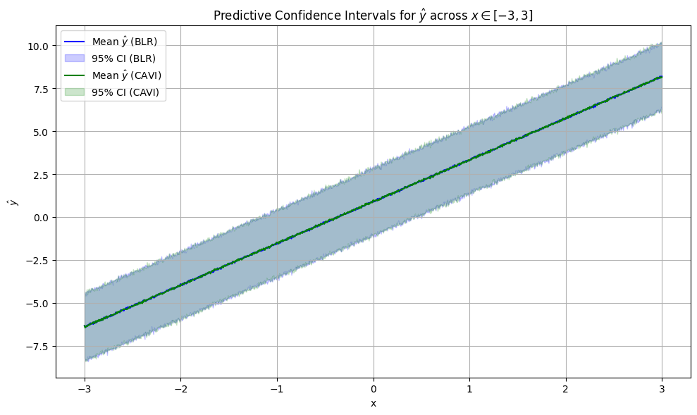
and … the predicted means and predictive confidence intervals are nearly identical again (at every point!), meaning that the CAVI algorithm has successfully modeled the true posterior. Truth be told, CAVI doesn’t always work this well. Many things were working in our favor here, which we list below:

1. We assumed to know the correct value of our residual variance \(\sigma^2\), as opposed to estimating it.
2. Our assumption that \(\beta_0\) and \(\beta_1\) are independently and normally distributed are 100% correct (by design, see our generate_data function.)
3. We used a sufficiently large number of samples ($n = 1000$), which is always helpful.
4. We used a sufficiently large number of parameter samples from the posterior (i.e. $K = 1000$) to compute our predictive distribution confidence intervals.

For fun, we can imagine what would happen if we didn’t take #4 above for granted. How would the (empirical) confidence intervals for predictions look if we sampled less parameters from the posterior? We create the satisfying fun video to show just that for values of \(K\) from two to 1000:

code

I have put all the code used for this blog post on this GitHub repo. Most of the code shown in this blog post is located in blr.py and cavi.py.

resources

Writing this piece required a lot of scavenging the web. Here’s my sources:

1. Notation on BNNs largely follows this piece from the University of Toronto.
2. For understanding Bayesian Linear Regression and deriving the exact posterior of \(\beta\) check out these class slides from University of Toronto’s CSC 411 and this Medium article.
3. For understanding variational inference, see this review paper or these notes from Princeton’s COS597C (both from Dr. Blei!). Additionally, these slides from CMU’s 10-418 explain CAVI in depth.

If you find this piece helpful, please cite this blog post below:

@article{bnns-cavi-versus-blr,
  title   = {What if we didn't approximate posteriors?},
  author  = {Lakkapragada, Anish},
  year    = {2025},
  month   = {May},
  url     = {https://anish.lakkapragada.com/blog/2025/bnn/}
}

Thank you for reading this blog post. If you have any questions or noticed any errata, please email me.