exponential family discriminant analysis

TLDR: Generalizing the Linear Discriminant Analysis (LDA) procedure to settings in which data in each class are all distributed according to the same exponential family distribution. Then testing this procedure with one such distribution, the Weibull.

Hey all! Hope you are doing well as usual. I am hoping in this somewhat more involved blog post to

• (1) give a brief overview of Linear Discriminant Analysis (LDA) and its relation to Logistic Regression
• (2) generalize LDA to settings in which our data is distributed according to an exponential family distribution
• (3) test our generalization in (2) with some toy datasets.

We start with an introduction to LDA.

a primer on linear discriminant analysis

Note: While LDA and Logistic Regression can be extended to be used for multiple classes, we focus solely on binary classification in this post.

Linear Discriminant Analysis (LDA) is a classification technique which models the distribution of data conditional on its class (i.e. \(X \mid Y\)), so as to create a (Bayes) classifier that models \(Y \mid X\). First note that this is in contrast to Logistic Regression, which directly models \(Y \mid X\). Let us establish some preliminaries: supppose we have covariates \(X = (x_1, \dots, x_p) \in \mathbb{R}^p\) and binary response \(Y \in \{0, 1\}\). Our end goal is to model \(p(X) = \mathbb{P}[Y = 1 \mid X]\), as it is well known that a classifier \(h\):

is a Bayes Classifier¹. For logistic regression, \(p(X)\) has the following form:

for learnable parameters \(\beta \in \mathbb{R}^{p + 1}\). For LDA, however, this is done through Bayes Rule. Let us define \(f_0(x)\) and \(f_1(x)\) as the PDFs of \(X \mid Y = 0\) and \(X \mid Y = 1\) respectively, and \(\alpha = \mathbb{P}[Y = 1]\), or the marginal probability of \(Y = 1\) across all data. LDA then gives the following form for \(p(X)\):

\begin{equation} p(X) = \mathbb{P}[Y = 1 \mid X] = \frac{\mathbb{P}[X \mid Y = 1] \mathbb{P}(Y = 1)}{\mathbb{P}[X \mid Y = 1] \mathbb{P}(Y = 1) + \mathbb{P}[X \mid Y = 0] \mathbb{P}(Y = 0)} = \frac{\alpha f_1(x)}{\alpha f_1(x) + (1 - \alpha) f_0(x)} \label{p-x} \end{equation}

Thus, LDA’s job is to learn \(f_0(x), f_1(x),\) and \(\alpha\) so as to model \(p(X)\). To do so, it assumes that \(X \in \mathbb{R}^p\) has a normal distribution for each class with a shared covariance matrix \(\mathbf{\Sigma} \in \mathbb{R}^{p \times p}\). Restated, LDA posits:

Thus to model \(f_0(x)\) and \(f_1(x)\), LDA learns parameters \(\mathbf{\mu_{1}}, \mathbf{\mu_{0}}, \mathbf{\Sigma}\) (and \(\alpha\)) through MLE on the given dataset \(\mathcal{D} = \{ (X_i, Y_i) \}_{i = 1}^{n}\). The MLEs are given below:

where \(N_1\) and \(N_0\) are the number of observations in \(\mathcal{D}\) belonging to class one and zero respectively.

We conclude this section with providing some understanding of the commonalities and differences between logistic regression and LDA. We start by giving the log-odds ratio of the LDA:

We can see that the log-odds ratios in LDA are modeled as a linear function of \(x\) (hence the name Linear Discriminant Analysis²). Furthermore, these coefficients in LDA can be thought of as parametrized versions of the logistic regression parameters \(\beta\).

In a nutshell, LDA offers a clean closed-form solution in exchange for strong parametric assumptions. Logistic regression gives us the opposite.

exponential family discriminant analysis

The achilles heel of the LDA is that it requires the strong assumption that observations in each class follow a normal distribution with shared covariance. So what if we could perform the LDA procedure but for all sorts of distributions? In this blog post, we aim to do exactly that for distributions falling under an exponential family.

exponential family: an abbreviated introduction

An exponential family is a set of probability distributions whose PDF \(f(\mathbf{x} \mid \mathbf{\eta})\) can be expressed as (using multivariable notation):

Before we explain the meaning of these functions in this seemingly strange PDF, it is important to stress that many common distributions we work with (e.g. $\mathcal{N}$, $\chi^2$, $\Gamma$) all fall under the exponential family. We now discuss two of these functions in our exponential family PDF:

• \(T(\mathbf{x}) \in \mathbb{R}^d\) (for some \(d \in \mathbb{N}\)) is the sufficient statistic. In words, this means that \(T(\mathbf{x})\) holds all information about parameter $\mathbf{\theta}$. In math, the conditional distribution \(\mathbf{x} \mid T(\mathbf{x})\) does not depend at all on $\mathbf{\theta}$.

• \(\mathbf{\eta} \in \mathbb{R}^d\) is the natural parameter. For our purposes, it is a convenient re-expression of \(\mathbf{\theta}\) amenable to this form (meaning that we have some (ideally invertible) function \(\mathbf{\theta} \mapsto \mathbf{\eta}\)).

The remaining functions \(A(\mathbf{\eta}) \in \mathbb{R}\) and \(h(\mathbf{x}) \in \mathbb{R}\) are not too important for our purposes other than to just make sure that \(f(\mathbf{x} \mid \mathbf{\eta})\) is a valid PDF (the former can be thought of as a normalization constant). There is a lot more to the exponential family. Feel free to read the Wikipedia page and these advanced notes I found for a much more thorough discussion.

discriminant analysis for exponential family data distributions

Having established all background requisite knowledge, we are ready to understand how we can generalize LDA to data with class-conditional distributions in the exponential family. With a slight abuse of terminology³, let us call this new procedure we are outlining as exponential family discriminant analysis (EFDA).

We start with our assumptions. We assume we have two classes of data where data in class one and zero are distributed according to respective exponential family PDFs \(f_1(\mathbf{x} \mid \mathbf{\eta}_1)\) and \(f_0(\mathbf{x} \mid \mathbf{\eta}_0)\) such that:

First note that PDFs \(f_1\) and \(f_0\) only differ by their true (natural) parameter values \(\mathbf{\eta}_1\) and \(\mathbf{\eta}_0\). To perform classification for EFDA, we aim to model \(p(X)\) in the same way we did for LDA (see \eqref{p-x}). Thus, we must estimate through MLE the parameters \(\alpha, \mathbf{\eta}_1,\) and \(\mathbf{\eta}_0\). We now derive these MLEs, starting with our log-likelihood function:

From the derivations below, you can see that the MLEs for $\mathbf{\eta}_1$ and $\mathbf{\eta}_0$ do not have a general closed-form solution. This is because the function $A(\mathbf{\eta})$ will differ among distributions in the exponential family. For example, $A(\mathbf{\eta}) = e^{\mathbf{\eta}}$ for the Poisson distribution but $A(\mathbf{\eta}) = \log(1 + e^{\mathbf{\eta}})$ for the Bernoulli distribution. As such, the best we can do is give a condition for these MLEs, which we present below (boxed):

We are now ready to test EFDA with a simulation.

worked example: weibull distribution

We now test EFDA in practice. For this example, let us assume that our data in each class is distributed according to the Weibull, which does have an exponential family parametrization. We can express this distribution as \(\text{Weibull}(\lambda, k)\), where parameters \(\lambda > 0\) (scale) and \(k > 0\) (shape). Moreover, the Weibull PDF can be given by \(f(x) = \frac{k}{\lambda} (\frac{x}{\lambda})^{k - 1} \exp(-(\frac{x}{\lambda})^k)\) for \(x \geq 0\). We now state our assumptions for our data in each class:

Recall that our goal with EFDA is to be able to learn \(\lambda_1\) and \(\lambda_0\), as well as \(\alpha = \mathbb{P}[Y = 1]\), so as to be able to model classifier function \(p(X) = \mathbb{P}[Y = 1 \mid X]\). For this simulation, we specify the following ground truth values:

Note that \(\alpha = 0.7\) means that there is an overall bias towards data belonging in class one. We provide the following plot below to understand the distributions of our different data:

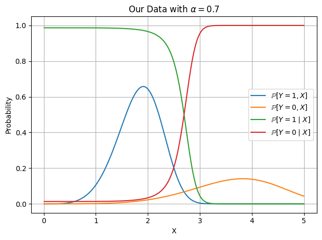
While the above plot can feel slightly overwhelming, I would recommend pausing to make sure each curve makes sense. From it, we can see that roughly something like \(x = 2.5\) seems to be a good barrier between data in class one (left) and data in class zero (right). As a bit of foreshadowing, we’ll also compute the log-odds ratio for our data:

and so the log-odds ratio are not a linear function of \(X\). We now proceed to actually use our derived EFDA procedure to model \(p(X)\) (green curve) from our given dataset \(\mathcal{D} = \{(X_i, Y_i)\}_{i = 1}^n\). As a first step, we give the exponential family parametrization of the Weibull PDF, for when \(k\) is known a priori:

For a verification that this does indeed work see below:

Recall that we are assuming that the true natural parameters \(\eta_1\) and \(\eta_0\) are different across each class. Now applying the derived MLE conditions stated in \eqref{efda-mle} for this specific exponential family parametrization, we can find the MLEs of \(\eta_1\) and \(\eta_0\). We start by deriving the former:

and so by identical logic we have:

Thus, we now have all the necessary ingredients to perform EFDA on our given dataset. We first start by giving the code to generate samples from our data:

CLASS_ONE_TRUE_LAMBDA = 2
CLASS_ZERO_TRUE_LAMBDA = 4
ALPHA_TRUE = 0.7
K_TRUE = 5 # common across both classes

def generate_data(n_samples): 
    X_class_one = weibull_min.rvs(c=K_TRUE, scale=CLASS_ONE_TRUE_LAMBDA, size=n_samples, random_state=42)
    X_class_zero = weibull_min.rvs(c=K_TRUE, scale=CLASS_ZERO_TRUE_LAMBDA, size=n_samples, random_state=42)
    y = (np.random.uniform(0, 1, size=n_samples) <= 0.7).astype(int) 
    X = y * X_class_one + (1 - y) * X_class_zero
    return X, y 

As a baseline, we’ll want to compare EFDA’s results to those of Logistic Regression. While we can’t do a direct comparison of their parameters (as they are inherently different), we’ll be interested in seeing how they model the log-odds differently. Specifically, across a number of different trials (each with different sampled datasets), we’ll want to see how Logistic’s Regression and EFDA’s log-odds ratio varies as a function of \(X\). We provide this plot below, across 100 different trials each with sample size \(n = 10^4\):

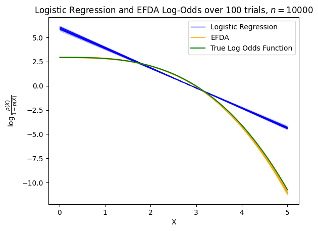
The major takeaway from this plot is that in cases where the true log-odds function is nonlinear (green curve), Logistic Regression will fail to model this nuance whereas a correctly-specified EFDA classifier will be able to. Furthermore, because Logistic Regression can only model the log-odds linearly, this means that for certain values of \(x\) (e.g. small \(x\)), it will overconfidently predict one class, and for other values of \(x\) (e.g. large \(x\)), it will underconfidently predict the other class.

further considerations

While EFDA did work quite well for this example with the Weibull distribution, note that it is not always guaranteed to do so. For instance, depending on the required \(A(\mathbf{\eta})\) function, the MLE conditions in \eqref{efda-mle} do not always lend themselves to a closed-form solution. As an example, the chi-squared exponential family parametrization necessitates \(A(\eta) = \log \Gamma(\eta + 1) + (\eta + 1)\log2\). Such a parametrization has an unwieldly derivative w.r.t \(\eta\) and likely will not have a closed-form solution for the MLE. Furthermore, EFDA, similar to LDA, suffers from the same strong assumption of a priori knowledge of the distribution of data in each class. Not to mention that this distribution must be the same among each class. As such, EFDA should be thought of as a bespoke solution with nice properties.

code

All code for the Weibull example can be found in this file.

resources

I list all my sources for this article below.

1. For a great introduction to LDA & QDA, please see these slides from Yale’s S&DS 242.
2. For understanding the exponential family for single and multivariate parametric sets, Wikipedia was of much help.

If you find this piece helpful, please cite this blog post below:

@article{exponential-family-discriminant-analysis,
  title   = {Exponential Family Discriminant Analysis},
  author  = {Lakkapragada, Anish},
  year    = {2025},
  month   = {May},
  url     = {https://anish.lakkapragada.com/blog/2025/efda/}
}

Thank you for reading this blog post. If you have any questions or noticed any errata, please email me.