using the vc dimension & rademacher complexity

TLDR: Testing VC dimension & Rademacher complexity generalization error bounds for a simple perceptron and a rectangular classifier.

Hey all! I hope you are doing well as usual. Over the last week, I realized I’ve never really touched Statistical Learning Theory at all before, despite hearing about it a lot. So I got slightly curious and went through these (IMO very approachable) introductory lecture notes on statistical learning theory by Dr. Cynthia Rudin for MIT’s 15.097.

What I found was that the theory yielded these really magical probabilistic bounds on generalization error, whereas the actual computation of these bounds was treated as an afterthought. Specifically, many of these bounds rested on some clever mathematical formalization of the capacity of the function class, such as the VC Dimension or the Rademacher Complexity. In this blog post I hope to explore how to compute these two quantities in actual function class examples. Doing so means that we can concretely test the VC & Rademacher generalization error bounds themselves.

establishing some preliminaries

notation

Please at least skim this section as notation for statistical learning theory is quite unconsistent across different places.

We start by defining some notation we’ll need for this blog post, most of which is directly taken from the 15.097 notes. We define our input space as \(\mathcal{X}\) and our output space as \(\mathcal{Y} = \{-1, 1\}\). Our observed data \(\{(X_i, y_i)\}_{i = 1}^m\) are drawn IID from distribution \(D\) on the space \(\mathcal{X} \times \mathcal{Y}\). Our goal is to create a function \(f: \mathcal{X} \to \mathcal{Y}\) that minimizes the true risk \(R^{\text{true}}(f) = \mathbb{P}_{(X, y) \sim D}[f(X) \neq y]\). Often times this risk is uncomputable as \(D\) is unknown and so we must settle by using the empirical risk \(R^{\text{emp}}(f) = \frac{1}{m} \sum_{i = 1}^m \mathbf{1}\{f(X_i) \neq y_i\}\).

There’s a vast range of functions we could think of that can map \(\mathcal{X} \to \mathcal{Y}\). As such, we’ll often constrain the empirical risk minimizer function we are searching for to a subset of all those functions, or a function class. Some function classes you are probably familiar with are linear models or 2-layer neural networks.

Sometimes, we won’t care about the predictions themselves (i.e. the output of \(f\)), but instead whether they were right or not. For a given function \(f: \mathcal{X} \to \mathcal{Y}\), we can define its loss function \(g: \mathcal{X} \times \mathcal{Y} \to \{0, 1\}\) as the following: \(g(x, y) = \mathbf{1}\{f(x) = y\}\). We can essentially think as the loss function a vehicle to assess the performance of another function (in fact, there is a bijection between \(g\) and \(f\)). For a given function class \(\mathcal{F}\), we can define the loss class \(\mathcal{G}\) as:

which is the set of all loss functions corresponding to all functions in our function class. We can also define the true & empirical risk easily with \(g\):

Lastly, note that we define the \(\text{sign}(\cdot)\) function as the following:

our function classes

To start, we’ll want to actually settle on what function classes we want to play around with. For this blog post, we’ll test two function classes. For each function class, we will test the VC & Rademacher bounds by generating a dataset from some ground-truth reality. We now provide these two function classes, along with the ground-truth parameters we will use for our simulations (boxed):

1. Linear Threshold Functions: \(\mathcal{F}_1 = \{x \mapsto \text{sign}(\mathbf{w}^Tx) \mid \mathbf{w} \in \mathbb{R}^2\} \quad \boxed{\mathbf{w} = (1, -2)}\)

2. Rectangle Classifiers: \(\mathcal{F}_2 = \{(x_1, x_2) \mapsto \text{sign}(\mathbf{1}\{a \leq x_1 \leq b \} \wedge \mathbf{1}\{c \leq x_2 \leq d \}) \mid (a, b, c, d) \in \mathbb{R}^4 \} \quad \boxed{(a, b, c, d) = (1, 3, 2, 4)}\)

Note that functions in the first function class \(\mathcal{F}_1\) lack a bias term, but are valid functions for our purposes nonetheless. You might also recognize \(\mathcal{F}_1\) to essentially be a class of binary classification perceptrons. The second function class \(\mathcal{F}_2\) is a bit more strange – essentially it posits data in class \(1\) inside a finite 2D rectangle with bottom left corner \((a, c)\) and top right corner \((b, d)\), and data in class \(-1\) as outside this rectangle. One commonality between both these function classes is they are uncountable¹, and thus well-suited for VC & Rademacher bounds.

While the VC & Rademacher Bound apply for any function in our function class \(\mathcal{F}_k\), we’ll be most interested in the function \(f_n = \underset{f \in \mathcal{F}_k}{\text{argmin}} \ R^{\text{emp}}(f) \in \mathcal{F}_k\), or the minimizer of the empirical risk. This is because \(f_n\) is the actual function in our function class we would use. It would be helpful then to understand how we actually would learn or at least estimate \(f_n\) for our two function classes. We detail the procedures below for each function class:

1. Learning \(\mathbf{w} \in \mathbb{R}^2\) for \(\mathcal{F}_1\)

To learn the weights for this perceptron, we’ll use the … perceptron algorithm, which is very simple. Suppose we have dataset \(\{(X_i, y_i)\}_{i = 1}^m\). We first start by setting \(\mathbf{w} \leftarrow \mathbf{0} \in \mathbb{R}^2\). Note that our goal is to ensure that \(\forall 1 \leq i \leq m, \ y_i\mathbf{w}^TX_i \geq 0\), as this indicates a correct classification. Thus, at every iteration of this algorithm, if for our \(i\)th sample \(y_i\mathbf{w}^TX_i < 0\), then we will set² \(\mathbf{w} \leftarrow \mathbf{w} + y_iX_i\).

This algorithm is so simple in code:

def learn_perceptron(X, y, iters):
    w = np.zeros(2) # initialize weights
    for _ in range(iters):
        for xi, yi in zip(X, y):
            if yi * np.dot(w, xi) <= 0: # wrong 
                w += yi * xi # update
    return w

2. Learning \((a, b, c, d)\) for \(\mathcal{F}_2\)

Using the assumption that most of our data’s class \(1\) observations can be fit into a finite 2D rectangle, we can simply choose \((a, b, c, d)\) by looking at the maximum and minimum x & y-coordinates of observations in class \(1\). In practice we won’t use the maximum & minimum, but instead the 95th & 5th percentile. Defining some dataset \(\{((h_i, v_i), y_i)\}_{i = 1}^m\) for this task³, we estimate our parameters as the following:

We are now ready to measure our function class’s capacity.

understanding our function class’s vc dimension

For a formal definition and construction of the VC Dimension, please see these lecture slides. I do not define it here.

Actually proving the VC Dimension for a function class can be quite tricky, as to conclude that a function class has VC dimension \(h\) one must show that there exists a set of \(h\) points that our function class can shatter and that no set of \(h + 1\) points exists that can be shatterable. The good news is that both of our defined function classes have established VC dimensions. For our first function class, the VC Dimension is two (as we are in \(\mathbb{R}^2\)), and for our second function class the VC Dimension is four.

While deriving the VC Dimension for our perceptron is quite hard (done here if our perceptron had a bias), understanding the VC Dimension for our rectangular class is slightly easier. See the next paragraph if interested.

Consider any four points in the plane - for every prediction configuration⁴, we can construct a rectangle such that only points of class \(1\) are inside. To conclude that the VC Dimension is four, though, we must show that it is not five. This can be seen from the fact that for any 5 points, we can intuitively expect one of those points to be the “interior”. Then setting the other four as all class \(1\) and this “interior” point as class \(-1\), no such rectangle can be made to accurately capture this prediction configuration without labeling the interior point as class \(1\). Thus the number of dichotomies made by \(\mathcal{F}_2\) on any five points is always \(< 2^5 \implies\) the growth function \(\neq 2^5 \implies\) the VC Dimension is \(< 5\). This concludes our extremely informal proof that the VC Dimension of \(\mathcal{F}_2\) is four.

We now present the VC Bound on generalization error, which we will actually test later. Suppose we have a function class \(\mathcal{F}\) with VC Dimension \(h\), and our data follows a distribution \(D\). Under this setup, we will draw training data \(\mathbf{Z} = \{(X_1, Y_1), \dots, (X_m, Y_m) \}\) from distribution \(D^m\), where \(m \geq h\). Then the VC Bound says \(\forall \delta > 0\):

\begin{equation} \mathbb{P}_{\mathbf{Z} \sim D^m}[\forall f \in \mathcal{F} : R^{\text{true}}(f) \leq R^{\text{emp}}(f) + 2\sqrt{2 \frac{h \log \frac{2em}{h} + \log \frac{4}{\delta}}{m}}] \geq 1 - \delta \label{vc-bound} \end{equation}

Note that the probability here stems from the randomnes of our training data, which will affect the empirical risk quantity.

estimating the rademacher complexity

For a very thorough treatment of Rademacher Complexity, way above my paygrade, see these lecture notes.

We now move to another approach to measuring the capacity of a function class, Rademacher Complexity. This approach is distribution dependent, and so it will focus on data from our actual distribution. This is in contrast to VC Dimension, which only concerned itself with the existence of any possible points being shatterable. Defining the Rademacher Complexity is a two-step process. Suppose we have a fixed dataset \(\mathbf{Z} = \{(X_i, Y_i)\}_{i = 1}^m \overset{\text{IID}}{\sim} D^m\) of \(m\) points, where \(D\) is our data distribution. We first give the Empirical Rademacher Complexity $\mathcal{\hat{R}_m(F)}$ of function class \(\mathcal{F}\):

where \(\sigma_1, \dots, \sigma_m\) are IID Rademacher random variables. Then, the Rademacher complexity \(\mathcal{R_m(F)}\) of \(\mathcal{F}\) is given by another expectation:

This expectation is over \(\mathbf{Z} \sim D^m\), or the \(m\)-sized dataset draws. In brief, the main idea of Rademacher complexity is that function classes which can fit random noise better have more capacity. Before explaining how we will actually estimate this \(\mathcal{R_m(F)}\) quantity, we’ll quickly present why we care about it (i.e. the Rademacher bound⁵):

Back to now estimating this Rademacher complexity term. The first thought might be a grid sampling procedure (i.e. first sample \(\mathbf{Z}\) and then \(\mathbf{\sigma}\)) and then try to compute the innermost \(\underset{f \in \mathcal{F}}{\sup} \frac{1}{m} \sum_{i = 1}^m \sigma_i f(X_i)\) term (more on that later.) While this is not a bad idea, I’m just a bit wary about how many iterations or trials it would take. Instead, we can cheat a little and just estimate the Empirical Rademacher Complexity Term. This is because we have a really nice generalization error bound involving just the empirical complexity:

\begin{equation} \forall \delta > 0, \mathbb{P}_{\mathbf{Z} \sim D^n}[\forall f \in \mathcal{F} : R^{\text{true}}(f) \leq R^{\text{emp}}(f) + \mathcal{\hat{R}_m(F)} + 3\sqrt{\frac{\log \frac{2}{\delta}}{m}}] \geq 1 - \delta \label{emp-rad-bound} \end{equation}

Estimating \(\mathcal{\hat{R}_m(F)}\) is not nearly as daunting. Given some random realization of \(m\) data points \(\{X_i\}_{i = 1}^m\), all we have to do is repeatedly across \(T\) trials sample Rademacher variables \(\sigma_1, \dots, \sigma_m\). Then for each trial, we train a model in our function class with our original data with corresponding labels \(\sigma_1, \dots, \sigma_m\). For this trained function \(f^*\), the summation \(\frac{1}{m} \sum_{i = 1}^m \sigma_i f^*(X_i) = \underset{f \in \mathcal{F}}{\sup} \frac{1}{m} \sum_{i = 1}^m \sigma_i f(X_i)\). Averaging these \(\frac{1}{m} \sum_{i = 1}^m \sigma_i f^*(X_i)\) quantities across each of our \(T\) trials will lead to an estimate for \(\mathbb{E}_{\mathbf{\sigma}}[\underset{f \in \mathcal{F}}{\sup} \frac{1}{m} \sum_{i = 1}^m \sigma_i f(X_i)] = \mathcal{\hat{R}_m(F)}\).

So there we have it! A way to estimate (for any function class!) the (empirical) Rademacher complexity.

testing out our bounds!

Now that we have generalization error bounds \eqref{vc-bound} and \eqref{emp-rad-bound}, let’s actually test them for our function classes.

\(\mathcal{F}_1\): binary classification perceptron

We train our perceptron on \(m_{\text{train}} = 10^4\) data points. While \(R^{\text{true}}(f)\) is pretty much unknowable, we’ll still want to estimate it. To do so, we approximate \(R^{\text{true}}(f)\) by evaluating our trained model on a test set of \(m_{\text{test}} = 10^4\) data points. We call this approximation \(R^{\text{test}}(f)\).

The below plot shows, at each iteration, \(R^{\text{test}}(f)\) and the 95% VC & Rademacher Bounds⁶ on \(R^{\text{true}}(f)\):

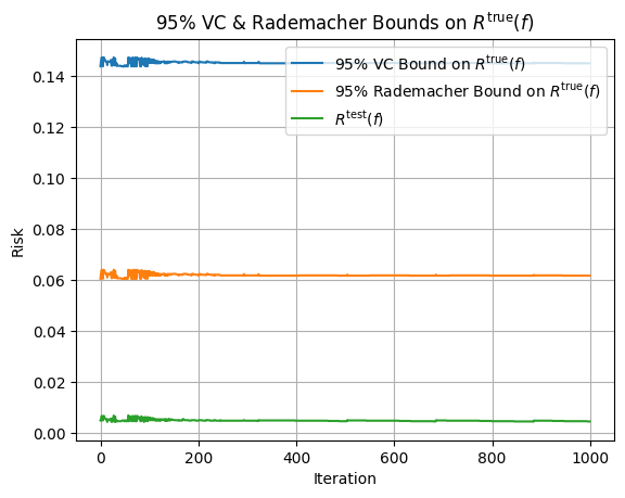
Right off the bat, we can see that although no bound appears particularly tight when compared to our estimate of \(R^{\text{true}}(f)\) (green curve), the VC Bound appears to be more than two times more conservative than the Rademacher bound. The unfortunate reality is that while the VC & Rademacher bounds provide formal justifications for the relationships between model complexity and overfitting, they are often too useless to be actually meaningful. The reason that we had to set \(m_{\text{train}}\) so high is that for datasets on the size of \(10^2\), the VC Bound was $>1$, which is completely useless as \(R^{\text{true}}(f) \leq 1\).

\(\mathcal{F}_2\): rectangular classifier

This function class is slightly different than the first as it is not iteratively learned. Unfortunately, that means we won’t have any pretty plots. We proceed with the same setup of \(m_{\text{train}} = m_{\text{test}} = 10^4\) and report the bounds:

• \(R^{\text{test}}(f)\) estimate of \(R^{\text{true}}(f)\): 0.0071
• 95% Rademacher Bound on \(R^{\text{true}}(f)\): 0.0640
• 95% VC Bound On \(R^{\text{true}}(f)\): 0.1903

Once again, we see that our bounds are still too conservative, with the VC bound being more than 3x the Rademacher bound.

code

The code for the two function classes can be found here.

resources

This blog post drew from a good amount of sources. I highly recommend the 15.097 notes as a place to start understanding Statistical Learning Theory. After that, here are some further places to go:

1. For understanding the VC dimension of our two function classes, see these slides from Purdue’s ECE 595.

2. For understanding the Rademacher complexity bounds (and seeing their derivations), feel free to take a look at the original paper presenting these bounds (Bartlett & Mendleson 2002) or these lecture notes from CMU’s 8803. Most of the notation I used when presenting Rademacher complexity was from the latter.

Thank you for reading this blog post. If you have any questions or noticed any errata, please email me.