supplement to the supplemental cs229 boosting lecture notes

TLDR: An exploration of a regularization alternative to the standard AdaBoost boosting algorithm. Then testing this regularization algorithm on same tree stump boosting classifer presented in the CS229 boosting lecture notes.

Hey all! Hope you are well and thank you for taking the time to check out this post. After spending nearly all of last month on Statistical Learning Theory bounds, I am ready to find something else to dig into. Having heard of boosting (and bagging) so much in statistical machine learning, I’ve been curious for a while now on what boosting really is. After reading through a few online sources on boosting, I really enjoyed these supplemental lecture notes on boosting from CS229. To the best of my knowledge, the notes’ “infinite feature function” perspective to boosting is unique and very clean to work with.

One thing the notes did not cover, though, was handling overfitting when boosting classifiers. While the boosting procedure is guaranteed to achieve zero training error eventually, it might not generalize as well as we would hope. In this really straightforward post, I’ll go over Gentle AdaBoost, or GentleBoost, an algorithm similar to AdaBoost that’s robust to overfitting. We’ll also test it on the same example presented in the original CS229 notes. In true supplement fashion, I’ll use the same notation as the original notes and only focus on binary classification¹. Because I won’t spend much time covering boosting theory, it’s probably worth skimming the notes if unfamiliar with AdaBoost (see Figure 2 in the notes).

an alternative to adaboost: gentleboost

motivation

AdaBoost is extremely sensitive to outliers (e.g. label noise). For an explanation why, consider the fact that outliers will tend to be the points learned last. Therefore, after a certain amount of iterations, the outliers’ weights \(p^{(i)}\) will be quite high and so AdaBoost will prioritize creating a weak classifier to satisfy these points. We now demonstrate this on the exact same CS229 decision stump boosting problem, with a twist: we’ll add 10% label noise to give AdaBoost room to overfit:

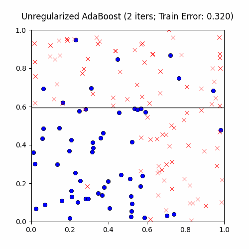
You can see that AdaBoost first creates sound, general decision boundaries before overfitting to the outliers with these cool islands encompassing a few points. True to its word, though, AdaBoost does at the end achieve zero training error.

gentleboost algorithm

The main difference in GentleBoost is that its weak-learning algorithm (WLA) is specified to give continuous predictions in the range of \([-1, 1]\), even if GentleBoost is trying to solve a classification problem. This makes GentleBoost more robust to outliers, as its weak-learners are “softer” with their predictions. We formally define the GentleBoost algorithm below, adapted from this paper:

Algorithm 1.1 – GentleBoost For Binary Classification

For each iteration \(t = 1, 2, \dots\):

(i) Define weights \(w^{(i)} = \exp(-y^{(i)} \sum_{\tau = 1}^{t - 1} \theta_{\tau} \phi_{\tau}(x^{(i)}))\) and distribution \(p^{(i)} = w^{(i)} / \sum_{j = 1}^m w^{(j)}\)

(ii) Use the given WLA to find \(\phi_t: \mathbb{R}^n \to [-1, 1]\) that minimizes the weighted least-squares error \(\sum_{i = 1}^m p^{(i)} (y^{(i)} - \phi_t(x^{(i)}))^2\)

(iii) Set \(\theta_t = \frac{1}{2}\).

For clarity, the final prediction on \(x\) after \(M\) iterations is given as \(\text{sign}(\sum_{\tau = 1}^{M} \phi_{\tau}(x))\).

It’s probably worth clarifying how we’ll adapt our decision stump WLA for GentleBoost. Whereas our decision stump \(\phi_{j, s}\) returned a binary classification earlier, now given some distribution \(p = (p^{(i)}, \dots, p^{(m)})\), we’ll define \(\phi_{j, s}: \mathbb{R}^n \to [-1, 1]\) as:

\[\text{left} = \{i: x_j^{(i)} < s \}, \quad \text{right} = \{i: x_j^{(i)} \geq s \}, \quad \phi_{j, s}(x) = \begin{cases} \frac{\sum_{i \in \text{left}} p^{(i)} y^{(i)}}{\sum_{i \in \text{left}} p^{(i)}} & \text{ if } x_j < s \\ \\ \frac{\sum_{i \in \text{right}} p^{(i)} y^{(i)}}{\sum_{i \in \text{right}} p^{(i)}} & \text{ if } x_j \geq s \end{cases}\]

As expected, our WLA will have to choose the best \(j\) and \(s\) to optimize the weighted least-squares objective. In comparison to our previous decision stump for AdaBoost, we can see this decision stump is less sensitive to outliers as its continuous prediction is OK with boundaries that possess some inconsistencies/outliers. This is also why GentleBoost is also a soft margin classifier² as it allows for some missclassifications in exchange for bigger margins (more on this later.)

While we’ll only test GentleBoost, note that there are also other variants of AdaBoost, such as RealBoost and Logit Boost. Before testing GentleBoost, we’ll shortly discuss another form of regularization: margins.

an aside: preventing overfitting with margins

Another way of preventing overfitting is through early stopping our boosting procedure before achieving zero training error. Doing so requires having some measurable criteria of when to stop training, or equivalently when meaningful training progress has stopped. One way that can be measured is the margin distribution across all samples. We first define a margin for a given sample:

Definition 1.2 – Margin of a Sample in a Boosting Classifier

Suppose we an infinite set of feature functions \(\phi = \{\phi_j\}_{j = 1}^{\infty}\), where each \(\phi_j: \mathbb{R}^n \to \{-1, 1\}\), and an infinite set of feature weights in vector \(\vec{\theta} = \begin{bmatrix} \theta_1 & \theta_2 & \dots \end{bmatrix}^T\). Then for a given observation \((x_i, y_i)\), we can define its margin \(\gamma_i\) as:

\[\gamma_i = y_i \frac{\theta^T \phi(x_i) }{\|\theta\|_1} = y_i \frac{\sum_{j = 1}^{\infty} \theta_j \phi_j(x_i)}{\sum_{j = 1}^{\infty} |\theta_j|}\]

So \(\lvert \gamma_i \rvert\) measures the distance between \(\hat{y}_i\) and the prediction decision boundary (i.e. prediction confidence) whereas \(\text{sign}(\gamma_i) > 0\) measures whether the prediction was correct or not. Suppose we have a dataset \(\{(x_i, y_i)\}_{i = 1}^m\) of \(m\) examples. Using these above definition of a per-sample margin, we can define the empirical margin distribution of our dataset to be \(\{\gamma_1, \dots, \gamma_m\}\). Note that we want our empirical margin distribution to place as much probability mass on positive, large values.

From there, there are plenty of ways to define the early stopping criteria. We could stop whenever the empirical margin distribution stops improving iteration by iteration. Alternatively, we could just boost until we achieve zero training error and select the model at the iteration where the empirical margin distribution was as left-skewed as possible.

testing gentleboost on our decision stump classification problem

We are now ready to actually compare GentleBoost vs. AdaBoost on our same decision stump problem, with 10% label noise. We first give the following GIF of the AdaBoost vs. GentleBoost decision boundaries across ~400ish iterations:

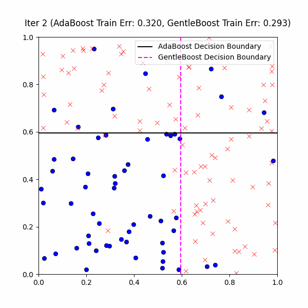
At first glance, it might look GentleBoost is not doing anything – after all, it is also creating these weird overfitting islands as well. However, if you look closely you’ll notice that GentleBoost consistently takes more iterations than AdaBoost before learning noise. This is made more clear in the the train/test error³ plot below over the first 10 iterations:

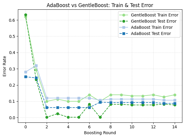
We can see that the lowest test error is clearly earned by GentleBoost. While overfitting inevitably happens as we train for 50+ iterations, GentleBoost offers a solid solution to at least putting some brakes to this problem.

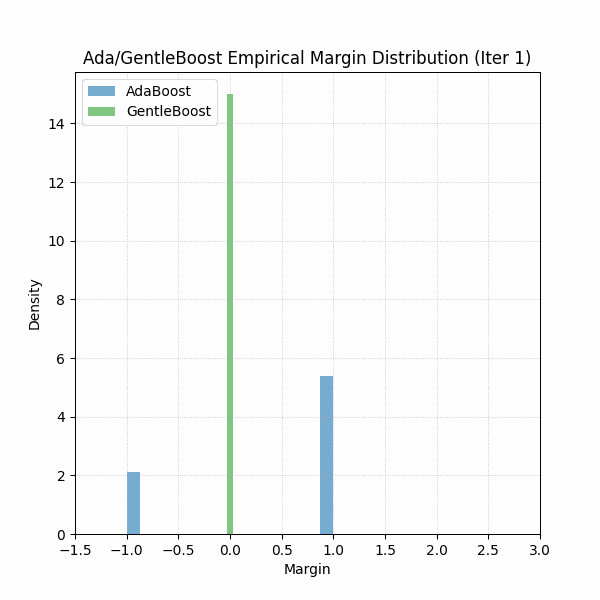
Furthermore, if you were curious about which algorithm’s margins were looking better, see GIF below for the first 30 iterations. Should be no surprise.

code

Unsanitized code for this repo can be found here.

resources

This post didn’t require as much source synthesis as others have in the past. The main source for this post was this paper from Stanford published in the Annals of Statistics. The paper is largely out of the scope of this post but provides good definitions for Gentle AdaBoost and other AdaBoost variants.

Thank you for reading this blog post. If you have any questions or noticed any errata, please email me.

1. We’ll continue using the standard \(\{-1, 1\}\) label space. ↩︎

2. This terminology is much more common when discussing SVMs. ↩︎

3. The test error is evaluated across 5000 generated datapoints with zero label noise. ↩︎