a quick tutorial of pac-bayesian and stability learning
the gentlest possible introduction to generalization error bounds beyond uniform convergence
TLDR: An abbreviated presentation of PAC-Bayesian and stability learning theory, with an example to test out generalization bounds. This post is a continuation of my previous post, which offers a much better overview of introductory statistical learning theory and uniform convergence bounds.
Hey there! I hope you are doing well. Admittedly, after my last blog post, I went on a bit of a statistical learning theory rabbit hole and tried to find something I could actually understand. While I definitely got stuck in a few dead ends, I managed to find through these old 2016 CS229T notes another interesting view of generalization bounds: that having higher capacity function classes wouldn’t affect overfitting if we didn’t use all of it. As overparametrized networks have been found to generalize great, I figured this kind of a view was important to take1. In particular, there are two methods that use this underlying view that I’d like to introduce and test today: PAC-Bayesian Learning and algorithmic stability.
understanding pac-bayesian learning
PAC-Bayesian learning is pretty straightforward. We break it into two steps. First, the PAC refers to the Probability Approximately Correct learning framework we are likely comfortable with. In particular, PAC learning provides us with the standard form of the generalization bound we all love:
\[\forall \delta > 0, \mathbb{P}_{\mathbf{Z} \sim D^n}[\forall f \in \mathcal{F}: R^{\text{true}}(f) \leq R^{\text{emp}}(f) + \text{Stuff}(\delta)] \geq 1 - \delta\]Note that this form of a bound (shared by VC Dimension, Rademacher Complexity, Covering Numbers, etc.) is of the uniform convergence flavor as it applies \(\forall f \in \mathcal{F}\). For the methods explored in this post, we’ll be looking at PAC bounds not of this type which, brushing aside a few technicalities, look like:
\[\forall \delta > 0, \mathbb{P}_{\mathbf{Z} \sim D^n}[R^{\text{true}}(f) \leq R^{\text{emp}}(f) + \text{Stuff}(\delta)] \geq 1 - \delta\]Now we move onto the Bayesian part. Suppose we have some classification function class \(\mathcal{F}\) (can be uncountable), and a “prior” distribution \(P\) over \(\mathcal{F}\). Then from our given data \(S \sim D^n\), we obtain some posterior distribution \(Q_s\) over \(\mathcal{F}\). Finally, we have some per-sample loss function \(\ell(f(x_i), y_i)\) which need not be the zero-one loss. Before establishing the important PAC-Bayesian generalization bound, let’s think about how we quantify risk in this case:
Definition 1.1 - Measuring Risk w.r.t to loss function \(\ell\)
Suppose we have some function class \(\mathcal{F}\) and some per-sample loss function \(\ell(f(x_i), y_i)\). Additionally we have some sample \(\{ (x_i, y_i)\}_{i = 1}^n\) of data drawn from data distribution \(D^n\). Then, for any function \(f \in \mathcal{F}\), we can define the following two respective quantities as the empirical and true risk of \(f\):
\[R^{\text{emp}}(f) = \frac{1}{n} \sum_{i = 1}^n \ell(f(x_i), y_i), \quad R^{\text{true}}(f) = \mathbb{E}_{(X, y) \sim D}[\ell(f(x), y)]\]Note that the latter quantity is often intractable as we assume \(D\) is unknowable. Now given some distribution \(Q\) over \(\mathcal{F}\), we can define the two following measures of risk of the distribution itself:
\[R^{\text{emp}}(Q) = \mathbb{E}_{h \sim Q}[R^{\text{emp}}(h)], \quad R^{\text{true}}(Q) = \mathbb{E}_{h \sim Q}[R^{\text{true}}(h)]\]
Essentially, we are now able to measure the training & true risk of not a function itself but of an entire distribution over the function class. With this definition, we can present the celebrated McAllester PAC-Bayesian learning bound:
Theorem 1.2 - McAllester’s PAC-Bayesian Learning Bound
For any prior \(P\) independent of the drawn data and all \(\delta \in [0, 1]\), we have the following bound:
\[\begin{equation} \mathbb{P}_{S \sim D^n}[\forall Q \ \text{on } \mathcal{F}: R^{\text{true}}(Q) \leq R^{\text{emp}}(Q) + \sqrt{\frac{\text{KL}(Q \mid\mid P) + \log \frac{2\sqrt{n}}{\delta}}{2n}}] \geq 1 - \delta \label{pac-bound} \end{equation}\]
This is intuitive enough to understand2 without a formal proof, as it appeals to familiar regularization idea: there is a tradeoff between the complexity of weights and the minimization of our empirical risk.
choosing data-dependent priors
If our goal is to minimize the RHS to yield the tightest possible bound on the true risk of our posterior distribution, there is one immediate step we can take. Consider the fact that even if \(\mathcal{F}\) is infinite, most of the possible choices are incredibly impractical given enough realizations of our data. For example, if we have function class \(\mathcal{F} = \{\text{sign}(w \cdot x + b) : w, b \in \mathbb{R}\}\) for data that roughly follows a line of \(y = \text{sign}(2x + 1)\), much of \(\mathcal{F}\) where \(w < 0\) or \(b < 0\) is entirely implausible. As such, a really uninformative prior over \(\mathcal{F}\) would be one like a MVN centered at \(w = b = 0\), as this prior is completely off the mark and thus driving up the \(\text{KL}(Q \mid\mid P)\) term in the RHS bound. Thus, we can use the following high-level strategy to tighten our bound:
Use some part of our dataset \(S\) to learn a prior \(P\) over \(\mathcal{F}\)
Learn a posterior \(Q_s\) over the remainder of our dataset. Then use \(Q_s\) and \(P\) to compute our McAllester generalization bound.
basic stability learning: uniform stability
A core idea of PAC-Bayesian Learning is that not every single function in our function class matters equally, which is why we have defined a posterior distribution over it. So it’s okay if we have an overparametrized function class if much of it holds zero mass in our posterior. Algorithmic stability is another flavor of statistical learning theory that also holds the same assumption: instead of looking at the capacity of the function class itself, algorithmic stability considers the stability of the learning procedure itself. High-capacity function classes aren’t a problem if the learning algorithm won’t willy-nilly explore all of it.
While there are many ways to define the stability of an algorithm in learning theory, we focus on one definition of uniform stability for this post. We now proceed to give the formal definition, copied from the CS229T notes.
Definition 2.1 - Uniform Stability
Let us first define \(\mathcal{Z}\) as the space in which our inputs lie3, \(D\) as our data distribution over \(\mathcal{Z}\), and \(\mathcal{H}\) is our hypothesis space. Suppose we have a learning algorithm \(\mathcal{A}: \mathcal{Z}^n \to \mathcal{H}\), where \(n\) is the number of points in our i.i.d input dataset has. Furthermore, for a given dataset \(S = (z_1, \dots, z_n)\), let us define the pertubation \(S^i = \{z'_i\} \cup \{ z_i : j \neq i \}\), where \(z'_i\) is an i.i.d replacement (i.e. \(z'_i \sim D\)) for the \(i\)th datapoint \(z_i\) in original dataset \(S\). Finally, we define a loss function \(\ell: (\mathcal{Z}, \mathcal{H}) \to \mathbb{R}\). Then we can say that \(\mathcal{A}\) has a uniform stability of \(\beta\) w.r.t loss function \(\ell\) if:
\[\forall S \in \mathcal{Z}^n, \forall S^i \in \mathcal{Z}^n, \forall z_o \in \mathbb{Z}: |\ell(z_0, A(S)) - \ell(z_0, A(S^i))| \leq \beta\]
The amount of \(\forall\) above should make you realize that this is quite a strong bound. Indeed, uniform stability is the strongest bar of stability and there are other weaker notions of stability. The main point of each of these stability notions is to arrive at generalization bounds, each of which are varyingly tight. We give the bound for uniform stability, adapted from Theorem 17 of the original Bousquet & Elisseeff (2002) paper:
Theorem 2.2 - Uniform Stability Generalization Error Bound
For a classification algorithm \(\mathcal{A}\) with uniform stability \(\beta\) w.r.t to loss function \(\ell\), we have the following probabilistic generalization error bound4:
\(\begin{equation} \forall \delta > 0, \mathbb{P}_{S \sim D^n}[R^{\text{true}}(A(S)) \leq R^{\text{emp}}(A(S)) + 2\beta + (4n\beta + 1)\sqrt{\frac{ \log \frac{1}{\delta}}{n}}] \geq 1 - \delta \label{stability-bound} \end{equation}\)
Fun stuff!
worked example: L2-regularized logistic regression
We are now ready to test out all these fun bounds in actual practice. We’ll do so with the L2-regularized logistic regression penalized by a fixed \(\lambda > 0\). We now begin setting up some definitions to give the L2-regularized logistic regression’s algorithm. First, we assume any given data observation \(x \in \mathbb{R}^d\) belongs to our data space \(\mathcal{X} \subset \mathbb{R}^d\) where \(\forall x_i \in \mathcal{X}, \|x_i\|_2 \leq R\) for some known constant \(R\). Second, we a priori restrict our logistic regression weights \(w \in \mathbb{R}^d\) to satisfy \(\|w\|_2 \leq \frac{R}{\lambda}\), which will be important later. We now define the per-sample loss function \(\ell(f, z)\) to be the logistic loss given below:
\[\ell(f, z) = \ell(f(x), y) = \log\left(1 + \exp(-y w^\top x)\right)\]The logistic loss above might feel a bit weird but it is essentially a modification of the standard binary cross-entropy loss for outputs in range \([0, 1]\) to our case where outputs are restricted from \([-1, 1]\). From this, we now present the dataset loss \(L_D(w, \lambda)\) which we will minimize:
\[L_D(w, \lambda) = \frac{1}{n} \sum_{i = 1}^n \ell(f(x_i), y_i) + \frac{\lambda}{2} \|w\|^2\]With this definition, we are ready to define our algorithm \(\mathcal{A}: (\mathbf{X}, y) \mapsto \mathbb{R}^d\) for L2-regularized logistic regression with a \(\lambda\) penalty:
\[\mathcal{A} = \underset{w \in \mathbb{R}^d}{\text{argmin}} \ L_D(w, \lambda)\]uniform stability of L2-regularized logistic regression
We’ll go backward and first start with the uniform stability of this model, with respect to our defined logistic loss function \(\ell(f(x), y)\). Luckily for us, a good amount of work has been done for us in this paper: the uniform stability of L2-regularized logistic regression is \(\frac{2\rho\tau}{\lambda n}\), where \(\ell(f(x), y)\) is \(\tau\)-Lipschitzian in the first argument and \(L_D(w, \lambda)\) is \(\rho\)-Lipschitzian in the first argument. If interested, see derivation below for \(\tau\) and \(\rho\).
Derivation of Lipschitzian Constants
For both these derivations, we use the fact that our a continuous differentiable function \(f\) is \(K\)-Lipschitz \(\iff \forall x, \| \nabla f(x) \|_2 \leq K\). We start by deriving \(\tau\) (note that \(\nabla\) and partial are same in univariate case):
\[\frac{\partial \ell}{\partial f(x)} = -y \frac{1}{1 + \exp(yf(x))} \implies | \frac{\partial \ell}{\partial f(x)} | = \frac{1}{1 + \exp(yf(x))} \leq 1\]and so we can use \(\tau = 1\). We go the same route for establishing a bound on \(\|\nabla_{w} L_D(w, \lambda) \|_2\):
\[\nabla_{w} L_D(w, \lambda) = \frac{1}{n} \sum_{i = 1}^{n} \frac{\partial \ell}{\partial f(x_i)} \nabla_{w} f(x_i) + \lambda w \implies \|\nabla_{w} L_D(w, \lambda) \|_2 \leq \frac{1}{n} \sum_{i = 1}^n \| x_i \|_2 + \lambda \| w\|_2 \leq 2R\]and so we can use \(\rho = 2R\).
We arrive at \(\tau = 1\) and \(\rho = 2R\). Thus, we can conclude the uniform stability of L2-regularized logistic regression w.r.t to \(\ell\) to be \(\boxed{\frac{4R}{\lambda n}}\) in our case. Plugging this result into \eqref{stability-bound}, we arrive at our nice uniform stability bound.
pac-bayesian learning using a naive prior
Recall that our bounds are slightly different here, as they measure the risk of a distribution \(R^{\text{true}}(Q)\) as opposed to the risk of a specific function \(R^{\text{true}}(h)\).
As a first stab at PAC-Bayesian Learning, we settle on using a completely uninformed prior. Our prior \(P\) and posterior \(Q_s\) are given below:
\[P \sim \mathcal{N}(\mathbf{0}, \sigma^2 I_d), \quad Q_s \sim \mathcal{N}(\hat{w}, \sigma^2 I_d)\]where \(\hat{w}\) is learned from \(\mathcal{A}\) and \(\sigma^2\) is pre-specified. The only term which is actually nasty to compute in the \eqref{pac-bound} bound is the \(\text{KL}(P \mid\mid Q_s)\) term. We use the formula provided here for multivariate Gaussians:
\[\text{KL}(P \mid\mid Q_s) = \frac{1}{2} [\log \frac{\det \Sigma_{Q_s}}{\det \Sigma_{P}} - d + (\mu_{P} - \mu_{Q_s})^T \Sigma_{Q_s}^{-1}(\mu_{P} - \mu_{Q_s}) + \text{trace}(\Sigma_{Q_s}^{-1} \Sigma_{P})]\] \[= \frac{1}{2}[\log(1) -d + \frac{1}{\sigma^2}\hat{w}^T\hat{w} + \text{trace}(I_d)] = \frac{\|\hat{w}\|_2^2}{2\sigma^2}\]pac-bayesian learning using an informed prior
The naive prior is obviously not the best. We partition our dataset \(S\) into two segments \(S_P\) and \(S_{Q}\). Then, we have \(\hat{w}_P = \mathcal{A}(S_P)\) and can construct the following prior \(P \sim \mathcal{N}(\hat{w}_P, \sigma^2 I_d)\). From there we use the dataset \(S_Q\) to independently learn \(\hat{w}_Q\) and establish the posterior \(Q \sim \mathcal{N}(\hat{w}_Q, \sigma^2 I_d)\). From doing so, we get that \(\text{KL}(Q \mid\mid P) = \frac{\|\hat{w}_Q - \hat{w}_P \|_2^2}{2\sigma^2}\). It might seem that this method would for sure lead to a tighter bound. However, keep in mind that now the amount of data points for the bound to be computed on is the size of \(S_Q\), which is less than the size of \(S\).
testing out our bounds
We are now ready to actually test out our bounds on L2-regularized Logistic Regression for the above discussed three approaches: (1) Uniform Stability (2) PAC-Bayes Naive and (3) PAC-Bayes Informed5. Our model will be for data in \(\mathbb{R}^5\), and we evaluate each of these bounds at 95% confidence or \(\delta = 0.05\). Furthermore, in order to make sure these bounds are tight6, we set \(\lambda = 0.1, R = 0.25\) and most importantly \(m = 10^6\).
For each of these approaches’ bounds, we also provide the measured7 empirical risk \(R^{\text{emp}}(f)\) or \(R^{\text{emp}}(Q)\). The gap between this measured empirical risk and its 95% bound on the true risk will tell us how tight our bounds are.
We first present a plot showing the uniform stability bound:
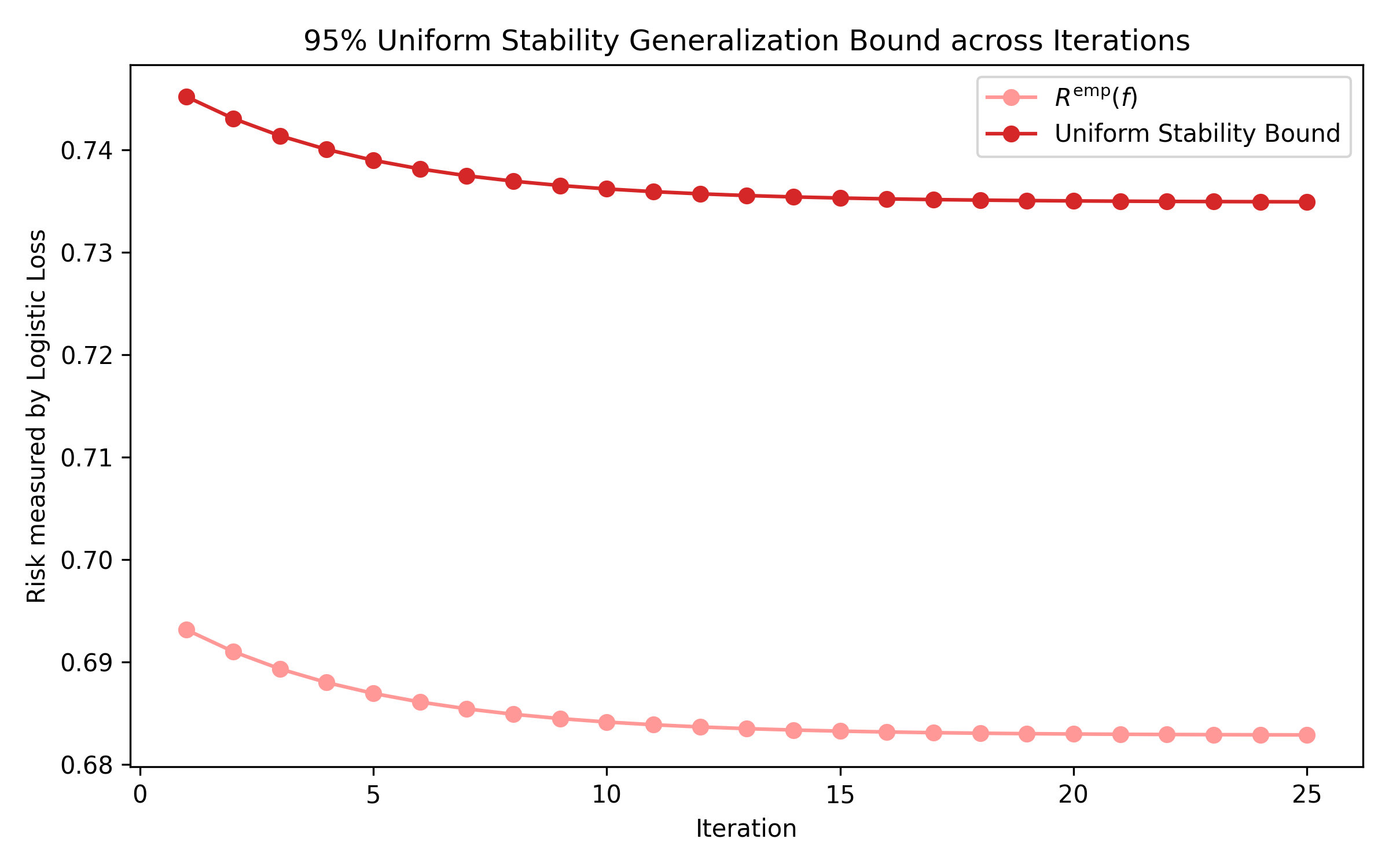
While this plot may not look terribly interesting, I don’t think it should be taken for granted. In our previous post the uniform convergence bounds, while not vacuous, were extremely useless. But here we are getting a 95% guarantee that our true risk is not \(\approx \frac{0.05}{0.68} = 7.35\)% greater than our measured empirical risk. IMHO, that’s quite useful and tangible.
We now provide the same plot for the PAC-Bayes generalization bounds, but in fun GIF form.

Looking at the scale of the vertical axis, we can see that these bounds are remarkably tight. Of all the generalization bounds I have actually computed in practice – VC Dimension, Rademacher, Uniform Stability, and now PAC-Bayes – PAC-Bayes has been the most tight. On the flip side, it is also the most tedious and computationally expensive. As an editorial comment, PAC-Bayes makes me very excited about Bayesian Machine Learning.
code
Running this code was extremely computationally expensive and so I had to use Colab for GPUs. Feel free to copy the Colab here and play around with some of the hyperparameters or code to generate your own figures!
resources
Writing this blog post as expected took a fair amount of meshing notationally inconsistent sources together. I list them below:
- The CS229T notes provided a very good introduction to PAC-Bayes and uniform stability. From there these slides went deeper into more modern & improved methods for PAC-Bayes.
- For understanding stability better (other than just uniform stability), please check the Bousquet & Elisseeff 2002 paper. These notes from UW’s CSE 522 also provide a good summary of stability learning bounds.
- Finally this paper on the stability of L2-regularized Logistic Regression (and of Decision Trees) were very helpful, as there is no way I could derive the uniform stability on my own.
Thank you for reading this blog post. If you have any questions or noticed any errata, please email me.
I’m obviously not the first person to have thought of this. Feel free to check these comprehensive slides on introducing PAC-Bayesian Learning presented at ICML 2019. ↩︎
This idea might seem very familiar to bayesian neural networks, in part because it is (there is a bijection between \(\mathcal{F}\) and the possible weights our function can take.) Note here that the cool part is getting a rich & rigorous generalization bound. ↩︎
Note that for this setup it is common that an input \(z \in \mathcal{Z}\) is really \(z = (x, y)\), where \(x\) is the data and \(y\) is the label. ↩︎
For this bound to mean anything, we want \(\beta = \mathcal{o}(\frac{1}{n})\). ↩︎
75% of the data is allocated towards learning the posterior. ↩︎
Because for \(\lambda > 0.1\) the model refused to learn (i.e. flat loss curves), to ensure meaningful bounds we had to largely compensate by increasing the amount of data points. It’s worth repeating that learning bounds are not actually meant to be numerically evaluated in practice, but I am curious and so we are doing so anyway. ↩︎
Note that for measuring \(R^{\text{emp}}(Q)\) we use an approximation by drawing weight/function samples \(f_1, \dots, f_{100} \sim Q\) and then computing \(\frac{1}{100} \sum_{i = 1}^{100} R^{\text{emp}}(f_i) \approx R^{\text{emp}}(Q)\). ↩︎