extending the black-scholes-merton constant volatility assumption

TLDR: A technical demonstration of why misspecified constant volatility can cause PnL drift even in delta-hedged portfolios. Then a brief presentation of some stochastic-volatility (SV) models/processes to extend the BSM.

I hope you are doing well! I apologize for not posting new blogs at my previous 1 post/week pace; I decided to take a break and instead spend that time going through the Green Book to learn more about all kinds of different stochastic processes. While many of my learnings did show up in my notes, I’m excited to present them now in a long-form post.

Specifically, in this blog post, I want to play around with the Black-Scholes-Merton model by taking a closer look at the implications of its constant volatility assumption. I was particularly inspired by this UChicago REU paper which presented different Stochastic Volatility (SV) processes; in this blog post, I hope to first demonstrate the risk of assuming constant volatility and end with some thorough exploration of these SV processes. I hope you enjoy.

introduction: setting up the bsm

I will assume some familiarity with Itô processes, SDEs, and Black-Scholes-Merton (BSM) in this post. For a thorough introduction into stochastic calculus, reference these solutions I’ve written.

As a reminder the BSM SDE posits that our stock-price \(S_t\) is given as a Geometric Brownian Motion under the risk-neutral measure¹:

\[dS_t = r S_t dt + \sigma S_t dW_t\]

where \(W_t\) is standard Brownian motion and \(\sigma\) is our constant volatility. From this SDE, we can derive the BSM PDE for our derivative \(V = V(S, t)\):

\[\frac{\partial V}{\partial t} + rS_t \frac{\partial V}{\partial S_t} + \frac{\sigma^2 S_t^2}{2} \cdot \frac{\partial^2 V}{\partial S_t^2} = rV\]

While a lot of things can be said about the BSM’s constant volatility assumption (e.g. volatility smile, which we’ll get into later), the bottom line is that it definitely affects the bottom line (i.e. PnL). We demonstrate this shortly after this quick disclaimer.

As pointed out by ChelseaFC here, it’s worth nothing that no model is ever perfect. For example, if we assume volatility to follow a GBM, we could (i) assume its volatility (i.e. volatility of volatility) to be constant or (ii) also model it with a stochastic process. We could go on like this forever. In short, a model without assumptions lacks ease-of-use; that being said, we will only focus on the constant volatilty assumption in this post.

demonstrating pnl drift in a delta-hedged portfolio

First suppose that our stock \(S_t\) does truly follow the below SDE for some true constant volatility \(\sigma\) and risk-free interest rate \(r\):

\[dS_t = r S_t dt + \sigma S_t dW_t\]

Now suppose we have a delta-hedged portfolio \(\Pi_t\):

\[\Pi_t = V_t - \Delta_t S_t + C_t\]

where we are (1) holding an option \(V_t\) (2) shorting \(\Delta_t := \frac{\partial V}{\partial S}(S_t,t)\) shares of \(S_t\) and (3) using the cash account \(C_t\) with a zero-investment strategy using self-financing & rebalancing². In particular for (3), a zero-investment strategy means \(\forall t, \Pi_t = 0 \implies C_t = -(V_t - \Delta_t S_t)\). Here’s what that means:

• If \(C_t > 0\), then we have cash on hand (\(\Delta_t S_t > V_t\)) which is being used to earn interest on.
• Otherwise, we are borrowing cash and paying interest.

Before going through \(d \text{PnL}\) (i.e. \(d\Pi_t\)), we’ll want to take a look at \(dC_t\) is. We’ll do this somewhat intuitively. Over time interval \([t, t + \delta]\) (\(\delta\) not to be confused with \(\Delta_t\)):

\[C_{t + \delta} = C_t(1 + r \delta) + S_t(\Delta_{t + \delta} - \Delta_t)\]

More or less what this means is that when there is a change in the delta \(\Delta_t\), we must adjust by that amount in terms of quantity of \(S_t\) (e.g. if \(\Delta_t \uparrow\) then we short more of \(S_t\) and so \(C_{t}\uparrow\)). The augend above reflects the fact that we are earning/borrowing at rate \(r\). From this discrete-time representation, it’s not too hard to see that:

\[dC_t = rC_t dt + S_t d\Delta_t\]

We are now ready to compute \(d\Pi_t\). Note that by the Itô product rule \(d(\Delta_t S_t) = \Delta_t dS_t + S_t d\Delta_t\) (see below for more details):

Derivation of differential of Short Quantity in Delta-Hedge

It is first worth recalling that \(\Delta_t = \frac{\partial V}{\partial S}(S_t, t)\) is an Itô process. Then by Itô Product rule, we have:

\[d(\Delta_t S_t) = \Delta_t dS_t + S_t d\Delta_t + d\langle \Delta, S_t \rangle_t\]

where \(d\langle \Delta, S_t \rangle_t\) is the quadratic covariation of the two processes. But since we typically think of \(\Delta_t\) as a limit of discrete changes (as we cannot update our portfolio in zero times), we asssume \(\Delta_t\) will have finite (total) variation \(\implies\) the quadratic covariation \(d\langle \Delta, S_t \rangle_t = 0\).

\[d\Pi_t = dV_t - d(\Delta_t dS_t) + dC_t = dV_t - \Delta_t dS_t - S_t d\Delta_t + rC_t dt + S_t d\Delta_t = dV_t - \Delta_t dS_t + rC_t dt\] \[= dV_t - \Delta_t dS_t - r(V_t - \Delta_t S_t) dt\]

We first try to get some understanding of \(dV_t\). Applying Itô’s Lemma we have:

\[dV_t = \frac{\partial V}{\partial t} dt + \frac{\partial V}{\partial S} dS_t + \frac{1}{2}\frac{\partial^2 V}{\partial S^2} (dS_t)^2.\]

Using the fact that \((dS_t)^2 = \sigma^2 S_t^2 dt\), we can simplify this to:

\[dV_t = \Big(\frac{\partial V}{\partial t} + rS_t \frac{\partial V}{\partial S} + \frac{1}{2}\sigma^2 S_t^2 \frac{\partial^2 V}{\partial S^2}\Big) dt + \frac{\partial V}{\partial S} \sigma S_t dW_t.\]

Substituting \(dV_t\) into \(d\Pi_t\) we get the following (recall what \(\Delta_t\) is):

\[d\Pi_t = \Big(\frac{\partial V}{\partial t} + rS_t \frac{\partial V}{\partial S} + \frac{1}{2}\sigma^2 S_t^2 \frac{\partial^2 V}{\partial S^2}\Big) dt + \frac{\partial V}{\partial S} \sigma S_t dW_t - \frac{\partial V}{\partial S} dS_t - rV_tdt + \frac{\partial V}{\partial S} rS_tdt\] \[= \Big(\frac{\partial V}{\partial t} + rS_t \frac{\partial V}{\partial S} + \frac{1}{2}\sigma^2 S_t^2 \frac{\partial^2 V}{\partial S^2}\Big) dt + \frac{\partial V}{\partial S} \sigma S_t dW_t - \frac{\partial V}{\partial S} [rS_t dt + \sigma S_t dW_t] - rV_t dt + \frac{\partial V}{\partial S} r S_t dt\] \[= \Big(\frac{\partial V}{\partial t} + rS_t \frac{\partial V}{\partial S} + \frac{1}{2}\sigma^2 S_t^2 \frac{\partial^2 V}{\partial S^2} - rV\Big) dt\]

Under the Black-Scholes Model we assume some volatility \(\sigma_*\) as the true constant volatility and have the following equation:

\[\frac{\partial V}{\partial t} + rS_t \frac{\partial V}{\partial S} + \frac{1}{2}\sigma_*^2 S_t^2 \frac{\partial^2 V}{\partial S^2} - rV = 0\]

Multiplying \(dt\) on both sides of this equation and then subtracting it from our derivation for \(d\Pi_t\) we have:

\[\boxed{d\Pi_t = \frac{1}{2}[\sigma^2 - \sigma_*^2] S_t^2 \frac{\partial^2 V}{\partial S^2}}\]

As per the Greeks convention, we’ll write \(\Gamma_t := \frac{\partial^2 V}{\partial S^2}(S_t, t)\). The main observation here is that when \(\Gamma_t > 0\), PnL drift works in our favor if the true volatility is greater than what we anticipated.

testing this out

To celebrate our hardwork, we’ll make a colorful visualization. Across a grid of values of the true volatility \(\sigma\) and our assumed BSM volatility \(\sigma_*\), we’ll generate a heatmap showing the estimated PnL at time \(t\):

\[\text{PnL}(t) = \int_{0}^{t} \frac{1}{2}[\sigma^2 - \sigma_*^2] S_t^2 \frac{\partial^2 V}{\partial S^2} dt\]

Heatmap shown below:

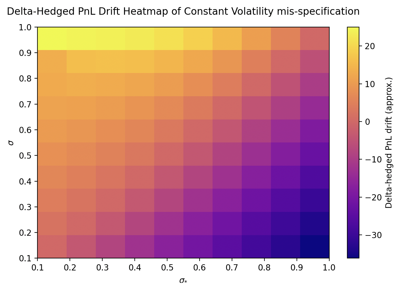
For unsanitized code that generated this, see here.

introducing some stochastic-volatility models

It’s worth repeating that the above was in the case that we had just misspecified the constant volatility – it was assuming the true volatility is constant. This is simply untrue. If we define the implied volatility as the calculated constant volatility that makes the BSM formula for a real-world option \(V_t\) equal its empirically observed price, we come across the following curve across various strike prices:

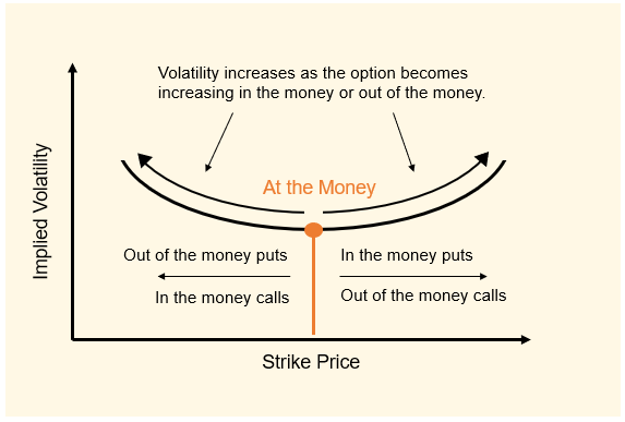
(Photo Credit). This curve is often called the volatility smile or volatility skew. So assumptions of constant volatility are clearly often wrong in practice. In response to this, there have been many developments of interesting models of stochastic volatility. Note that the math for using these models to evaluate an option \(V_t\) is way out of my wheelhouse (see Carr & Madam integrals). We’ll now take a look at a few of them.

updating volatility with shock observations: arch, garch(1, 1), ewma

These methods update the volatility based on weighting the history of the previous shocks (i.e. returns). Define \(u_i = \log(\frac{S_i}{S_{i - 1}})\) to give the shock from the \(i - 1\)th to the $i$th day/hour/etc. Also define \(V_L\) to be the long-run variance of the \(u_i\)’s (e.g. \(V_L = \mathbb{E}[u_i^2]\) as \(\mathbb{E}[u_i] = 0\)). We’ll explain how \(V_L\) is estimated soon. Then according to the ARCH model we have the following model (with \(m\) as a parameter) on our volatility \(\sigma^2_n\):

\[\boxed{\sigma^2_n = \gamma V_L + \sum_{i = 1}^{m} \alpha_i u_{n - 1}^2}\]

where \(\gamma + \sum_{i = 1}^m \alpha_i = 1\). We typically will estimate \(V_L\) over \(N \gg m\) observations: \(V_L \approx \frac{1}{N} \sum_{i = 1}^N u_{i}^2\). Note that this condition on \(\gamma\) and the \(\alpha_i\)’s lead to \(\mathbb{E}[\sigma^2_n] = V_L\) under this model; essentially we can think of \(V_L\) as the long-run volality/variance of our daily returns \(u_i\).

From the ARCH model, comes the Generalized ARCH (i.e. GARCH) model, which we give below for the \((1, 1)\) parametrization (hence denoted by GARCH(1, 1)):

\[\boxed{\sigma_n^2 = \gamma V_L + \alpha u_{n - 1}^2 + \beta \sigma_{n - 1}^2}\]

where \(\gamma + \alpha + \beta = 1\).

Finally, we give the exponentially weighted moving average (EWMA) model where we have:

\[\boxed{\sigma_{n}^2 = \lambda \sigma_{n - 1}^2 + (1 - \lambda) u_{n - 1}^2}\]

for some parameter \(\lambda \in [0, 1]\).

sv as an itô process: heston model

At high risk of sounding pretentious, this is the sine qua non of this post: SDEs for both \(S_t\) and its volatility. The Heston model gives the following SDE for the underlying stock price:

\[dS_t = \mu S_t dt + \sqrt{V_t} S_t dW_t^S\]

where our volatility \(V_t\) has the following SDE:

\[dV_t = \kappa(V_L - V_t) dt + \lambda \sqrt{V_t} dW_t^V\]

and \(W_t^S\) and \(W_t^V\) are two separate standard Brownian motions.

sources

To gain a better background in the kind of stuff, I think this UChicago REU Paper and the first few pages of these class notes would be helpful.

Thank you for reading this blog post. If you have any questions or noticed any errata, please email me.

1. For a proof on why we can use this SDE for \(S_t\) under BSM assumptions and a risk-free interest rate \(r\), see Proposition 1 in these notes. ↩︎

2. For our purposes, self-financing & rebalancing means all of our portfolio value is managed by the cash account (i.e. withdrawing money or lending money), as opposed to any outside deposits/withdrawals. ↩︎